Unit 2 Introduction

2.1 Working with data

rbind - combines data frames by stacking rows. Example:

#nrow gives number of rows
nrow(cars) # cars is a built-in dataset that comes with R; 

## [1] 50

dataframe1 <- cars # Assign cars to variable in environment
dataframe2 <- cars
boundframe <- rbind(dataframe2, dataframe1)
nrow(boundframe)

## [1] 100

2.1.1 Loading data files

WHO <- read.csv("week1/WHO.csv") #file hosted on EdX analytiics edge class
WHO_Europe = subset(WHO, Region == "Europe") #Subset data frame where Region is equal to Europe
write.csv(WHO_Europe, "week1/WHO_Europe.csv") #Write dataframe to csv file

2.1.2 Summary Statistics

str(WHO) #compactly displays the structure of a R object

## 'data.frame':    194 obs. of  13 variables:
##  $ Country                      : Factor w/ 194 levels "Afghanistan",..: 1 2 3 4 5 6 7 8 9 10 ...
##  $ Region                       : Factor w/ 6 levels "Africa","Americas",..: 3 4 1 4 1 2 2 4 6 4 ...
##  $ Population                   : int  29825 3162 38482 78 20821 89 41087 2969 23050 8464 ...
##  $ Under15                      : num  47.4 21.3 27.4 15.2 47.6 ...
##  $ Over60                       : num  3.82 14.93 7.17 22.86 3.84 ...
##  $ FertilityRate                : num  5.4 1.75 2.83 NA 6.1 2.12 2.2 1.74 1.89 1.44 ...
##  $ LifeExpectancy               : int  60 74 73 82 51 75 76 71 82 81 ...
##  $ ChildMortality               : num  98.5 16.7 20 3.2 163.5 ...
##  $ CellularSubscribers          : num  54.3 96.4 99 75.5 48.4 ...
...

summary (WHO) #Summary of object

##                 Country                      Region     Population     
##  Afghanistan        :  1   Africa               :46   Min.   :      1  
##  Albania            :  1   Americas             :35   1st Qu.:   1696  
##  Algeria            :  1   Eastern Mediterranean:22   Median :   7790  
##  Andorra            :  1   Europe               :53   Mean   :  36360  
##  Angola             :  1   South-East Asia      :11   3rd Qu.:  24535  
##  Antigua and Barbuda:  1   Western Pacific      :27   Max.   :1390000  
##  (Other)            :188                                               
##     Under15          Over60      FertilityRate   LifeExpectancy 
##  Min.   :13.12   Min.   : 0.81   Min.   :1.260   Min.   :47.00  
...

mean(WHO$Under15) #Mean of Under15 column

## [1] 28.73242

sd(WHO$Under15) #Standard Deviation of Under15 column

## [1] 10.53457

which.min(WHO$Under15) #Row conataining minimum value in Under15 column

## [1] 86

2.1.3 Plots

2.1.3.1 Scatter Plots

plot(WHO$GNI, WHO$FertilityRate)

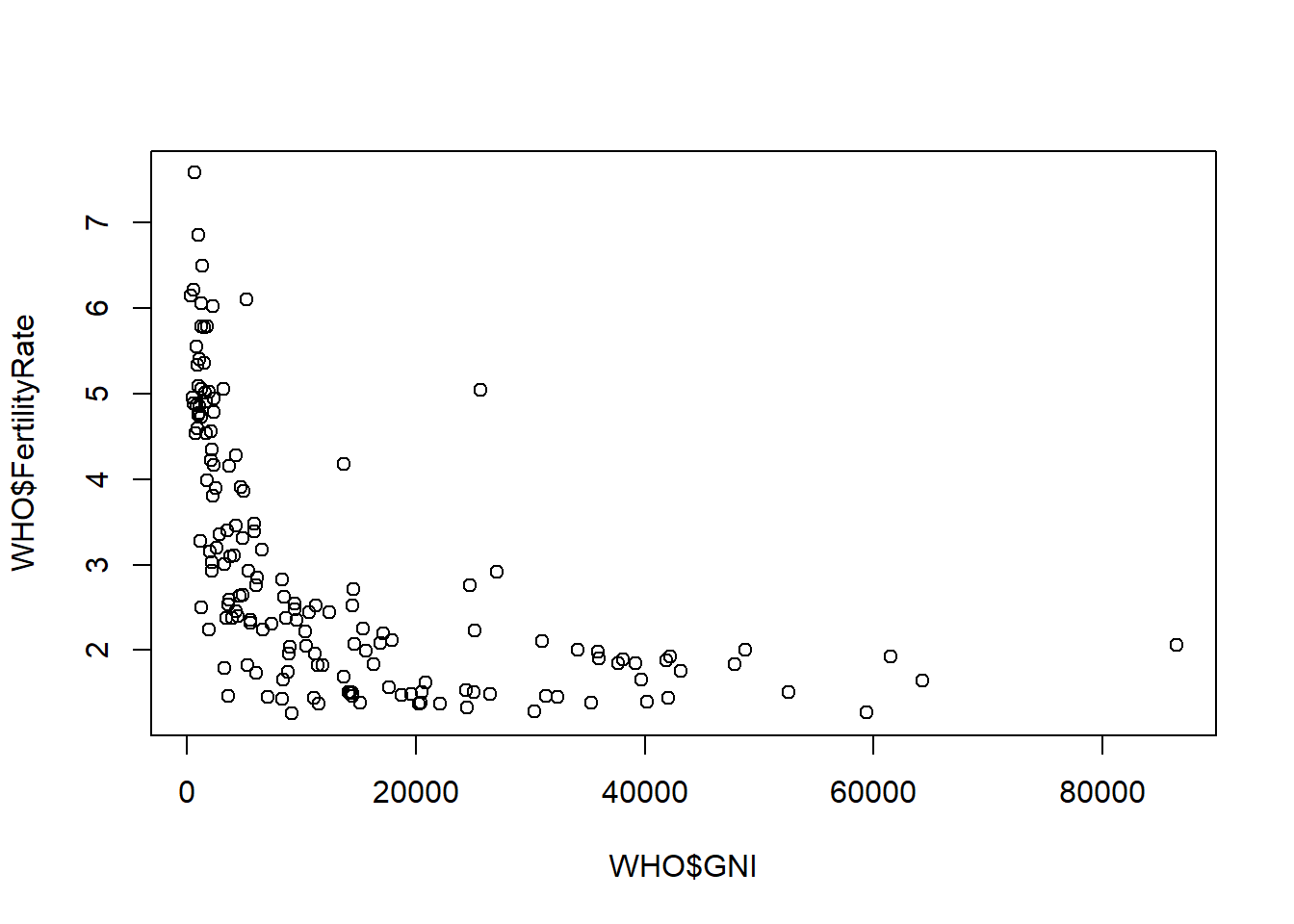
Outliers = subset(WHO, GNI>10000 & FertilityRate >2.5) # subset Outliers based on visual inspection of plot
Outliers[c("Country", "GNI", "FertilityRate")] # Subset 3 variables based on Outliers 

##               Country   GNI FertilityRate
## 23           Botswana 14550          2.71
## 56  Equatorial Guinea 25620          5.04
## 63              Gabon 13740          4.18
## 83             Israel 27110          2.92
## 88         Kazakhstan 11250          2.52
## 131            Panama 14510          2.52
## 150      Saudi Arabia 24700          2.76

2.1.3.2 Histograms

hist(WHO$CellularSubscribers) #Histogram

2.1.3.3 Box Plots

boxplot(WHO$LifeExpectancy ~ WHO$Region, xlab="Region", ylab="Life Expectancy")

2.1.4 Summary tables

table(WHO$Region) # Summary table; Works well for factor type variables

## 
##                Africa              Americas Eastern Mediterranean 
##                    46                    35                    22 
##                Europe       South-East Asia       Western Pacific 
##                    53                    11                    27

tapply(WHO$Over60, WHO$Region, mean) #table apply -- Find mean of over60 variable by Region

##                Africa              Americas Eastern Mediterranean 
##              5.220652             10.943714              5.620000 
##                Europe       South-East Asia       Western Pacific 
##             19.774906              8.769091             10.162963

tapply(WHO$LiteracyRate, WHO$Region, mean, na.rm=TRUE) #na.rm removes all missing values (NA) 

##                Africa              Americas Eastern Mediterranean 
##              69.09167              92.43529              82.52000 
##                Europe       South-East Asia       Western Pacific 
##              98.78077              71.78000              90.12222

2.2 Recitation - USDA Food Database

2.2.1 Data Analysis - Recitation

USDA <- read.csv("week1/USDA.csv")# file hosted on EdX
str(USDA)

## 'data.frame':    7058 obs. of  16 variables:
##  $ ID          : int  1001 1002 1003 1004 1005 1006 1007 1008 1009 1010 ...
##  $ Description : Factor w/ 7054 levels "ABALONE,MIXED SPECIES,RAW",..: 1303 1302 1298 2303 2304 2305 2306 2307 2308 2309 ...
##  $ Calories    : int  717 717 876 353 371 334 300 376 403 387 ...
##  $ Protein     : num  0.85 0.85 0.28 21.4 23.24 ...
##  $ TotalFat    : num  81.1 81.1 99.5 28.7 29.7 ...
##  $ Carbohydrate: num  0.06 0.06 0 2.34 2.79 0.45 0.46 3.06 1.28 4.78 ...
##  $ Sodium      : int  714 827 2 1395 560 629 842 690 621 700 ...
##  $ SaturatedFat: num  51.4 50.5 61.9 18.7 18.8 ...
##  $ Cholesterol : int  215 219 256 75 94 100 72 93 105 103 ...
...

summary(USDA)

##        ID       
##  Min.   : 1001  
##  1st Qu.: 8387  
##  Median :13294  
##  Mean   :14260  
##  3rd Qu.:18337  
##  Max.   :93600  
##                 
##                                                        Description  
##  BEEF,CHUCK,UNDER BLADE CNTR STEAK,BNLESS,DENVER CUT,LN,0" FA:   2  
...

names(USDA) # names of the variables in the data frame

##  [1] "ID"           "Description"  "Calories"     "Protein"      "TotalFat"    
##  [6] "Carbohydrate" "Sodium"       "SaturatedFat" "Cholesterol"  "Sugar"       
## [11] "Calcium"      "Iron"         "Potassium"    "VitaminC"     "VitaminE"    
## [16] "VitaminD"

match("CAVIAR", USDA$Description)# Find row which description matches CAVIAR

## [1] 4154

2.2.2 Histogram - Recitation

#Histogram - xlim sets limits for x-axis. breaks sets how many histogram bins
hist(USDA$VitaminC, xlab = "Vitamin C (mg)", main = "Histogram VItaminc C Lev.", xlim = c(0,100), breaks=2000)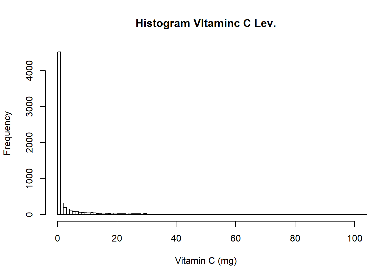 

2.2.3 Summary tables - Recitation

# Add 1 if  Sodium value greater than mean, and 0 if less
USDA$HighSodium <- as.numeric(USDA$Sodium > mean(USDA$Sodium, na.rm = TRUE)) #as.numeric converts the TRUE or FALSE to 1, or 0
USDA$HighProtein <- as.numeric(USDA$Protein > mean(USDA$Protein, na.rm = TRUE)) 
USDA$HighFat <- as.numeric(USDA$SaturatedFat > mean(USDA$SaturatedFat, na.rm = TRUE)) 
USDA$HighCarbs <- as.numeric(USDA$Carbohydrate > mean(USDA$Carbohydrate, na.rm = TRUE)) 
table (USDA$HighSodium, USDA$HighFat)

##    
##        0    1
##   0 3350 1332
##   1 1478  589

tapply(USDA$Iron, USDA$HighProtein, mean, na.rm=TRUE)

##        0        1 
## 2.558945 3.197294

2.3 Assignment

2.3.1 Part 1 - Analytical Detective

2.3.1.1 Problem 1

mvtWeek1 <- read.csv("week1/mvtWeek1.csv") 

Problem 1.1 - How many rows of data (observations) are in this dataset?

nrow(mvtWeek1)

## [1] 191641

Problem 1.2 - How many rows of data (observations) are in this dataset?

length(names(mvtWeek1))

## [1] 11

Problem 1.3 - Using the “max” function, what is the maximum value of the variable “ID”?

max(mvtWeek1$ID)

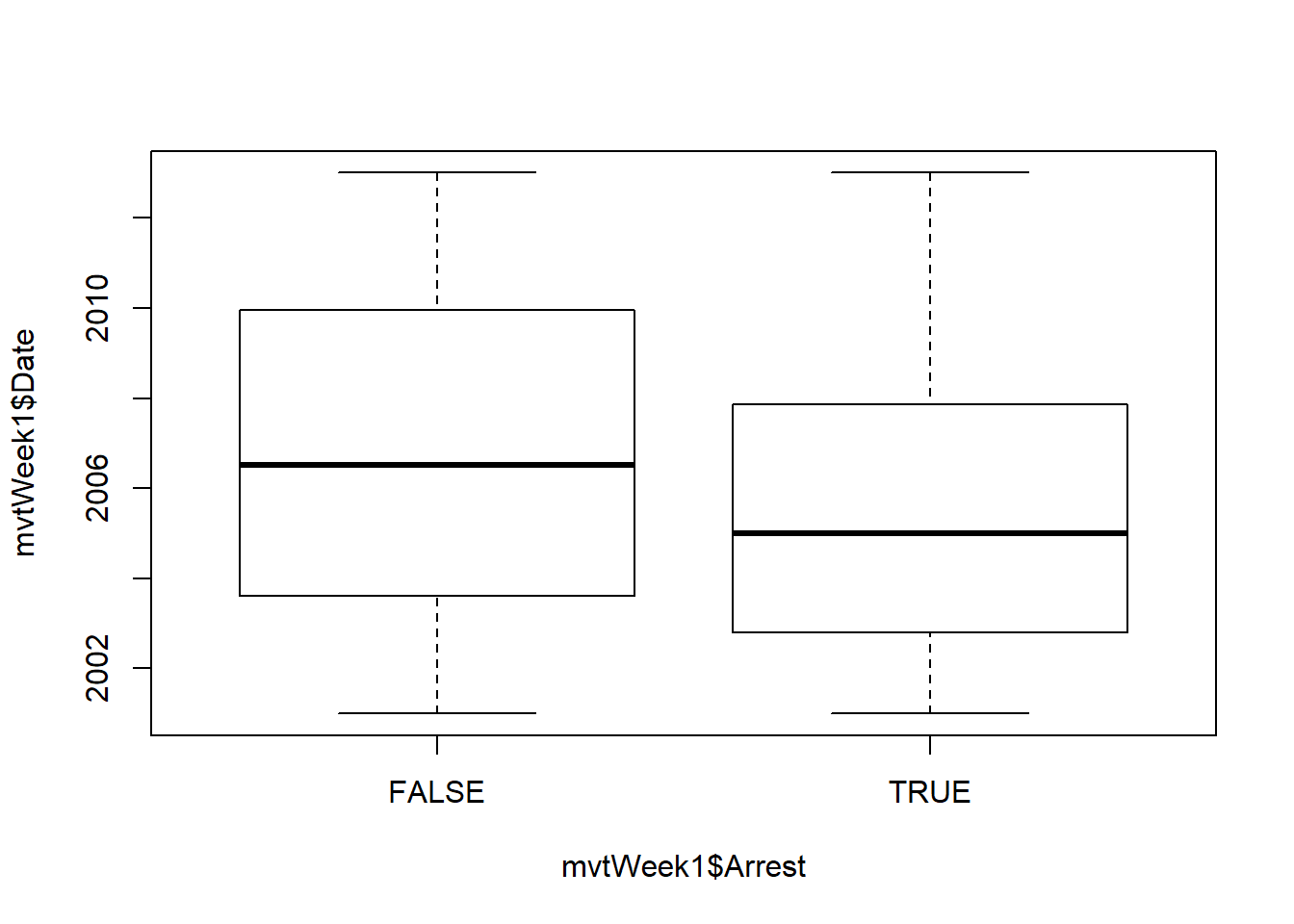
## [1] 9181151

Problem 1.5 - How many observations have value TRUE in the Arrest variable (this is the number of crimes for which an arrest was made)?

nrow(subset(mvtWeek1, Arrest == TRUE))

## [1] 15536

2.3.1.2 Problem 2

Problem 2.2 - Convert Date to Date Object in R

DateConvert <- as.Date(strptime(mvtWeek1$Date, "%m/%d/%y %H:%M")) #Original date format is Month/Day/Year Hour:Minute
head(DateConvert)

## [1] "2012-12-31" "2012-12-31" "2012-12-31" "2012-12-31" "2012-12-31"
## [6] "2012-12-31"

mvtWeek1$Month <- months(DateConvert)
mvtWeek1$Weekday <- weekdays(DateConvert)
mvtWeek1$Date <- DateConvert

Problem 2.3 - In which month did the fewest motor vehicle thefts occur?

which.min(table(mvtWeek1$Month))

## February 
##        4

which.max(table(mvtWeek1$Weekday)) #2.4

## Friday 
##      1

Problme 2.5 - Which month has the largest number of motor vehicle thefts for which an arrest was made?

#I plan to do some benchmarking on a large dataset to see which is more efficient
table(mvtWeek1$Arrest, mvtWeek1$Month) # Look at table for min ORR

##        
##         April August December February January  July  June March   May November
##   FALSE 14028  15243    15029    12273   14612 15477 14772 14460 14848    14807
##   TRUE   1252   1329     1397     1238    1435  1324  1230  1298  1187     1256
##        
##         October September
##   FALSE   15744     14812
##   TRUE     1342      1248

which.max(table(subset(mvtWeek1, Arrest == TRUE)$Month)) #Gives exact answer.

## January 
##       5

2.3.1.3 Problem 3

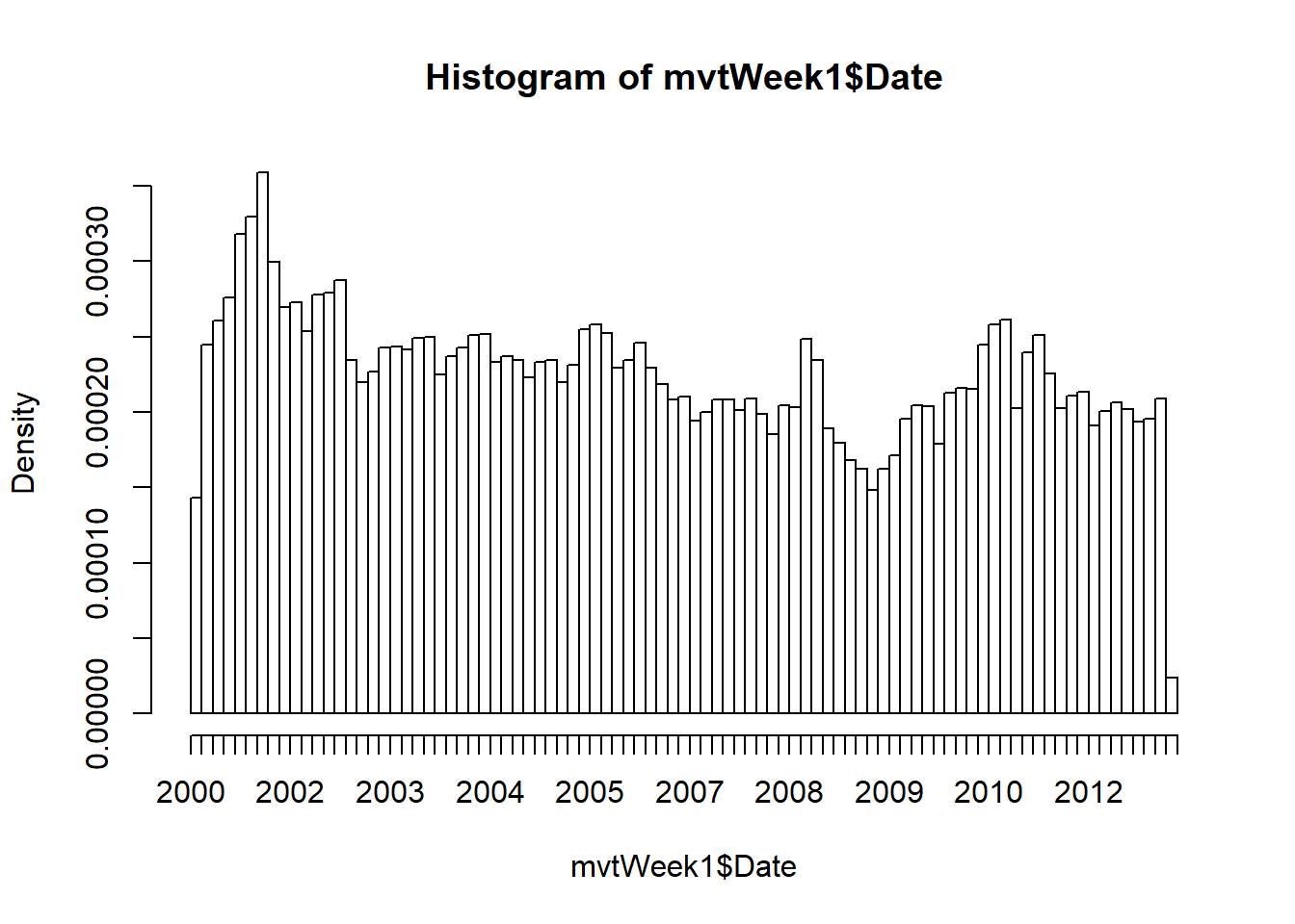
Problem 3.1 - Visualizing Crime Trends

hist(mvtWeek1$Date, breaks = 100)

boxplot(mvtWeek1$Date ~ mvtWeek1$Arrest)

2.3.1.4 Problem 4

Problem 4.1 - Which locations are the top 5 for motor vehicle thefts

sort(table(mvtWeek1$LocationDescription))

## 
##     AIRPORT BUILDING NON-TERMINAL - SECURE AREA 
##                                               1 
##                  AIRPORT EXTERIOR - SECURE AREA 
##                                               1 
##                                 ANIMAL HOSPITAL 
##                                               1 
##                                 APPLIANCE STORE 
##                                               1 
##                                       CTA TRAIN 
...

TopLocations = c("STREET", "PARKING LOT/GARAGE(NON.RESID.)", "ALLEY", "GAS STATION", "DRIVEWAY - RESIDENTIAL")
nrow(Top5<-subset(mvtWeek1, LocationDescription %in% TopLocations)) #Number of Obs. in Top5 Locations

## [1] 177510

2.3.2 Part 2 - Stock Dynamics

2.3.2.1 Read in csv files and convert dates

#####A lot of the problems get repetitive, so I’ll only include questions that intoroduce new functions or are interestng

IBM <- read.csv("week1/IBMStock.csv")
GE <- read.csv("week1/GEStock.csv")
ProcterGamble <- read.csv("week1/ProcterGambleStock.csv")
CocaCola <- read.csv("week1/CocaColaStock.csv")
Boeing <- read.csv("week1/BoeingStock.csv")

IBM$Date <- as.Date(IBM$Date, "%m/%d/%y")
GE$Date <- as.Date(GE$Date, "%m/%d/%y")
ProcterGamble$Date <- as.Date(ProcterGamble$Date, "%m/%d/%y")
CocaCola$Date <- as.Date(CocaCola$Date, "%m/%d/%y")
Boeing$Date <- as.Date(Boeing$Date, "%m/%d/%y")
min(rbind(Boeing,CocaCola,GE,IBM,ProcterGamble)$Date)# Problem 1.2

## [1] "1970-01-01"

2.3.2.2 Problem 1 - Standard deviation

sd(ProcterGamble$StockPrice) #Problem 1.8

## [1] 18.19414

2.3.2.3 Problem 2 - Visualizing Stock Dynamics

plot(CocaCola$Date, CocaCola$StockPrice, col="red")
lines(ProcterGamble$Date, ProcterGamble$StockPrice, col="blue") 
abline(v=as.Date(c("2000-03-01")), lwd=2) #abline adds straight line to a plot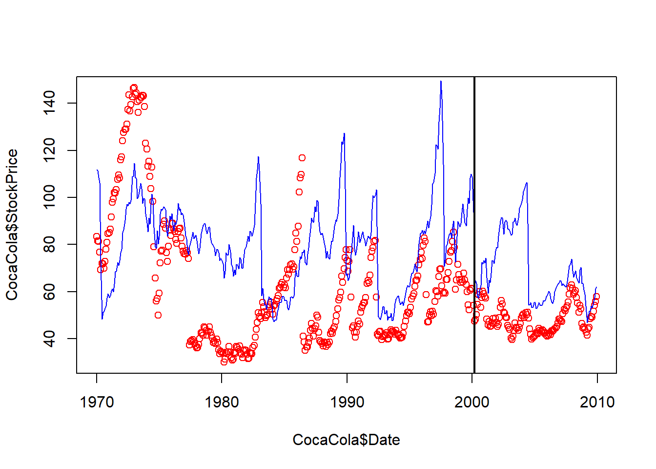

2.3.2.4 Problem 4- Monthly Trends

tapply(IBM$StockPrice, months(IBM$Date), mean)

##     April    August  December  February   January      July      June     March 
##  152.1168  140.1455  140.7593  152.6940  150.2384  139.0670  139.0907  152.4327 
##       May  November   October September 
##  151.5022  138.0187  137.3466  139.0885

2.3.3 Part 3 - Demographics and Employment in the United States

2.3.3.1 Problem 1 - Loading Data

CPS <- read.csv("week1/CPSData.csv") 
str(CPS)

## 'data.frame':    131302 obs. of  14 variables:
##  $ PeopleInHousehold : int  1 3 3 3 3 3 3 2 2 2 ...
##  $ Region            : Factor w/ 4 levels "Midwest","Northeast",..: 3 3 3 3 3 3 3 3 3 3 ...
##  $ State             : Factor w/ 51 levels "Alabama","Alaska",..: 1 1 1 1 1 1 1 1 1 1 ...
##  $ MetroAreaCode     : int  26620 13820 13820 13820 26620 26620 26620 33660 33660 26620 ...
##  $ Age               : int  85 21 37 18 52 24 26 71 43 52 ...
##  $ Married           : Factor w/ 5 levels "Divorced","Married",..: 5 3 3 3 5 3 3 1 1 3 ...
##  $ Sex               : Factor w/ 2 levels "Female","Male": 1 2 1 2 1 2 2 1 2 2 ...
##  $ Education         : Factor w/ 8 levels "Associate degree",..: 1 4 4 6 1 2 4 4 4 2 ...
##  $ Race              : Factor w/ 6 levels "American Indian",..: 6 3 3 3 6 6 6 6 6 6 ...
...

2.3.3.2 Problem 2 - Evaluating Missing values

table(CPS$Region, is.na(CPS$Married))

##            
##             FALSE  TRUE
##   Midwest   24609  6075
##   Northeast 21432  4507
##   South     33535  7967
##   West      26388  6789

sort(tapply(is.na(CPS$MetroAreaCode), CPS$State, mean)) #Proportion of NAs by State

## District of Columbia           New Jersey         Rhode Island 
##           0.00000000           0.00000000           0.00000000 
##           California              Florida        Massachusetts 
##           0.02048401           0.03923092           0.06492199 
##             Maryland             New York          Connecticut 
##           0.06937500           0.08060769           0.08568406 
##             Illinois             Colorado              Arizona 
##           0.11221881           0.12991453           0.13154450 
##               Nevada                Texas            Louisiana 
##           0.13308190           0.14370496           0.16137931 
...

mean treats boolean variables as 1s and 0s.

2.3.3.3 Problem 3- Integrating Metropolitan Area Data

MetroAreaMap <- read.csv("week1/MetroAreaCodes.csv") 
CountryMap <- read.csv("week1/CountryCodes.csv") 
str(MetroAreaMap)

## 'data.frame':    271 obs. of  2 variables:
##  $ Code     : int  460 3000 3160 3610 3720 6450 10420 10500 10580 10740 ...
##  $ MetroArea: Factor w/ 271 levels "Akron, OH","Albany-Schenectady-Troy, NY",..: 12 92 97 117 122 195 1 3 2 4 ...

Problem 3.2 Merge the Maps into CPS data frame to Replace the code with actual values

CPS <- merge(CPS, MetroAreaMap, by.x="MetroAreaCode", by.y="Code", all.x=TRUE) #all.x prevents NA observations froom being discarded
CPS <- merge(CPS, CountryMap, by.x="CountryOfBirthCode", by.y="Code", all.x=TRUE)
summary(CPS)

##  CountryOfBirthCode MetroAreaCode   PeopleInHousehold       Region     
##  Min.   : 57.00     Min.   :10420   Min.   : 1.000    Midwest  :30684  
##  1st Qu.: 57.00     1st Qu.:21780   1st Qu.: 2.000    Northeast:25939  
##  Median : 57.00     Median :34740   Median : 3.000    South    :41502  
##  Mean   : 82.68     Mean   :35075   Mean   : 3.284    West     :33177  
##  3rd Qu.: 57.00     3rd Qu.:41860   3rd Qu.: 4.000                     
##  Max.   :555.00     Max.   :79600   Max.   :15.000                     
##                     NA's   :34238                                      
##           State            Age                 Married          Sex       
##  California  :11570   Min.   : 0.00   Divorced     :11151   Female:67481  
...

sort(tapply(CPS$Race == "Asian", CPS$MetroArea, mean))

##                                         Albany, GA 
##                                        0.000000000 
##                                        Altoona, PA 
##                                        0.000000000 
##                                       Amarillo, TX 
##                                        0.000000000 
##                                       Anderson, IN 
##                                        0.000000000 
##                                        Appleton,WI 
##                                        0.000000000 
...